Feature selection helps improve the performance of machine learning models by identifying the most relevant and informative features in a dataset. By only selecting the most relevant features, data scientists can reduce the risk of overfitting, which can lead to poor performance on new data. Feature selection also helps to reduce the computational cost of training and prediction, which is especially important for large datasets.

Principal Component Analysis (PCA) and Linear Discriminant Analysis (LDA) are two of the feature selection methods.

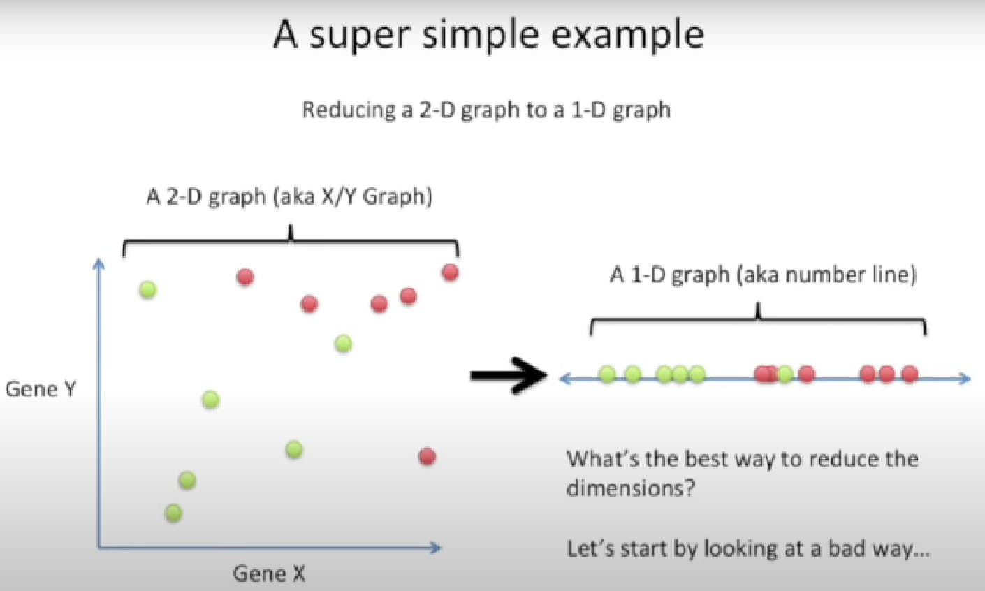
1. Principal Component Analysis (PCA): This is a dimensionality reduction technique that transforms the original features into a smaller set of uncorrelated features called principal components. The principal components are ranked based on their variance, and a subset of the top-ranked components is selected.

   PCA works by identifying a new set of orthogonal variables, called principal components, that capture the maximum amount of variation in the original data. The first principal component is the linear combination of the original variables that explains the largest amount of variance in the data. The second principal component is the linear combination that explains the second-largest amount of variance, and so on.

   

   The principal components are ordered by their variance, with the first component having the highest variance. By selecting only the top k principal components, where k is a user-defined parameter, we can reduce the dimensionality of the dataset from n to k, while retaining most of the original variation.

   Example

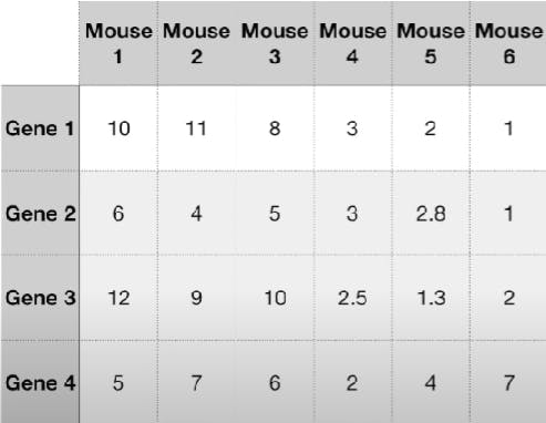
   Consider the following dataset:

   

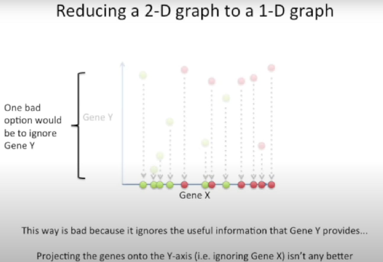
   If we consider only Gene 1 and plot it, we see:

   

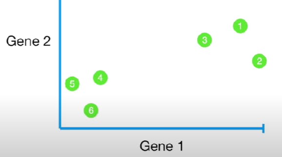
   Similarly, if we consider Gene 1 and 2, we see:

   

   We can also plot for Genes 1, 2, and 3:

   

   But if we consider the fourth gene too, it would be difficult to plot and visualize it. Here is where PCA comes into action!

   Let's consider only genes 1 and 2 to see how PCA works.

   First, calculate the average measurement for Genes 1 and 2. For gene 1, it is equal to (10+11+8+3+2+1)/6. For gene 2, it is (6+4+5+3+2.8+1)/6. Now plot this point in the graph.

   

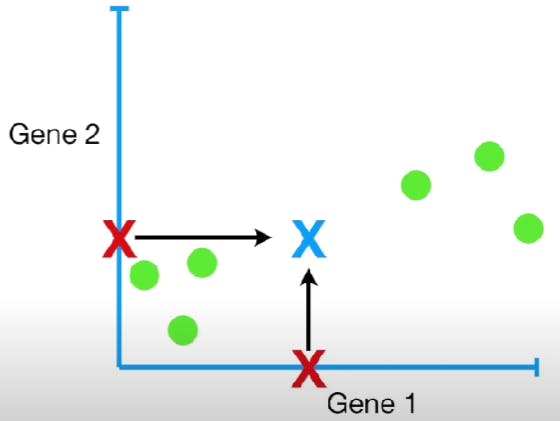
   Now we want to shift the data so that this new point is at the origin, and the relative positions of the other points are the same.

   Now plot a random line that goes through the origin. We want this line to be the best-fitting line of all the data points.

   

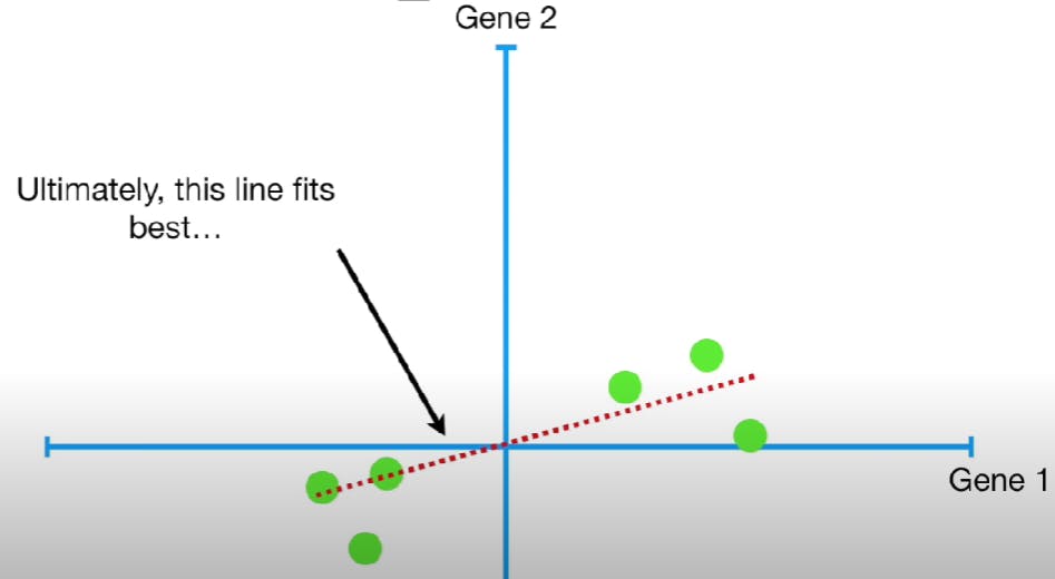
   The slope of this line is 0.25. i.e if we move four units in the Gene 1 axis, we have to move one unit in the Gene 2 axis. This means that the data points are mostly spread out along the Gene 1 axis, compared to the Gene 2 axis. Thus, Gene 1 is more important to know how the data is spread out. This red line is the PC1 line. Since this plot is 2D, the PC2 line is the line perpendicular to the PC1 line. Thus, its slope is -4. i.e if we move negative one unit on the Gene 1 axis, we have to move four units on the Gene 2 axis.

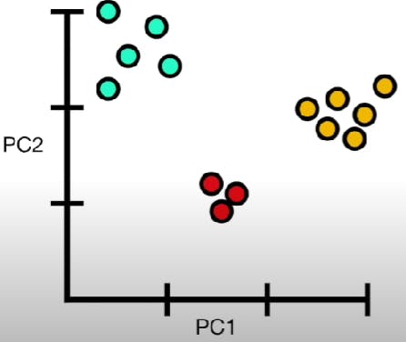
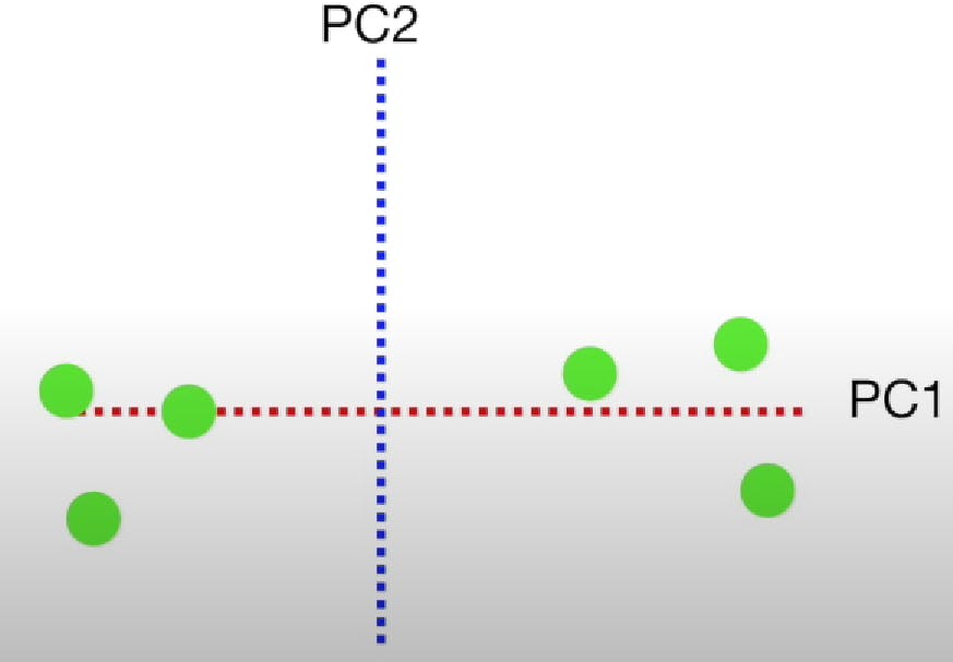
   To make the final plot, we rotate the plot such that the PC2 line becomes the Y-axis and PC1 becomes the X-axis.

   

Filter methods: These methods use statistical techniques to evaluate the relationship between each feature and the target variable. The features are ranked based on their relevance to the target variable, and a subset of the top-ranked features is selected. Linear Discriminant Analysis or LDA is one such method.

LDA is like PCA, but it focuses on maximizing the separability among known categories.

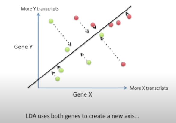
This new axis is created based on two criteria.

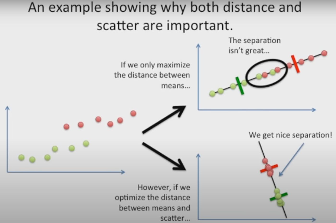
1) Maximization of the distance of the means of both categories.

2) Minimization of the variation within each category.

So, LDA focuses on creating an axis that maximizes the distance between the means for the two categories while minimizing the variation/scatter.

---

All the images were taken from the StatQuest Channel. Go check them out to learn about PCA and LDA in more depth!